45 how to change excel chart data labels to custom values

How to Change Excel Chart Data Labels to Custom Values? First add data labels to the chart (Layout Ribbon > Data Labels) Define the new data label values in a bunch of cells, like this: Now, click on any data label. This will select "all" data labels. Now click once again. At this point excel will select only one data label. Using the CONCAT function to create custom data labels for an Excel chart Use the chart skittle (the "+" sign to the right of the chart) to select Data Labels and select More Options to display the Data Labels task pane. Check the Value From Cells checkbox and select the cells containing the custom labels, cells C5 to C16 in this example.

Excel tutorial: How to customize axis labels Now let's customize the actual labels. Let's say we want to label these batches using the letters A though F. You won't find controls for overwriting text labels in the Format Task pane. Instead you'll need to open up the Select Data window. Here you'll see the horizontal axis labels listed on the right. Click the edit button to access the ...

How to change excel chart data labels to custom values

How to add or move data labels in Excel chart? - ExtendOffice In Excel 2013 or 2016. 1. Click the chart to show the Chart Elements button . 2. Then click the Chart Elements, and check Data Labels, then you can click the arrow to choose an option about the data labels in the sub menu. See screenshot: In Excel 2010 or 2007. 1. click on the chart to show the Layout tab in the Chart Tools group. See screenshot: 2. Then click Data Labels, and select one type of data labels as you need. See screenshot: Format Data Labels in Excel- Instructions - TeachUcomp, Inc. To format data labels in Excel, choose the set of data labels to format. To do this, click the "Format" tab within the "Chart Tools" contextual tab in the Ribbon. Then select the data labels to format from the "Chart Elements" drop-down in the "Current Selection" button group. Then click the "Format Selection" button that ... Apply Custom Data Labels to Charted Points - Peltier Tech Click once on a label to select the series of labels. Click again on a label to select just that specific label. Double click on the label to highlight the text of the label, or just click once to insert the cursor into the existing text. Type the text you want to display in the label, and press the Enter key.

How to change excel chart data labels to custom values. Modify Excel Chart Data Range | CustomGuide Select the chart Click the Design tab. Click the Select Data button. Select the series you want to change under Legend Entries (Series). Click the Edit button. Type the label you want to use for the series in the Series name field. Click OK. Click OK again. The name is updated in the chart, but the worksheet data remains unchanged. How to Change Axis Values in Excel - Excelchat Right-click on the chart and choose Select Data Click on the button Switch Row/Column and press OK Figure 11. Switch x and y axis As a result, switches x and y axis and each store represent one series: Figure 12. How to swap x and y axis The chart will have more logic if we track store values per years. Excel charts: how to move data labels to legend - Microsoft Tech Community You can't do that, but you can show a data table below the chart instead of data labels: Click anywhere on the chart. On the Design tab of the ribbon (under Chart Tools), in the Chart Layouts group, click Add Chart Element > Data Table > With Legend Keys (or No Legend Keys if you prefer) Custom data labels in a chart - Get Digital Help If you have excel 2013 you can use custom data labels on a scatter chart. 1. Right press with mouse on a series 2. Press with left mouse button on "Add Data Labels" 3. Right press with mouse again on a series 4. Press with left mouse button on "Format Data Labels" 5. Enable check box "Value from cells" 6. Select a cell range 7. Disable check box "Y Value"

How to add data labels in excel to graph or chart (Step-by-Step) 1. Select a data series or a graph. After picking the series, click the data point you want to label. 2. Click Add Chart Element Chart Elements button > Data Labels in the upper right corner, close to the chart. 3. Click the arrow and select an option to modify the location. 4. How to create Custom Data Labels in Excel Charts Two ways to do it. Click on the Plus sign next to the chart and choose the Data Labels option. We do NOT want the data to be shown. To customize it, click on the arrow next to Data Labels and choose More Options … Unselect the Value option and select the Value from Cells option. Choose the third column (without the heading) as the range. Custom Data Labels with Colors and Symbols in Excel Charts - [How To] To apply custom format on data labels inside charts via custom number formatting, the data labels must be based on values. You have several options like series name, value from cells, category name. But it has to be values otherwise colors won't appear. Symbols issue is quite beyond me. How to use cell values for excel chart labels - How to We want to chart the sales values and use the change values for data labels. Use Cell Values for Chart Data Labels. Select range A1:B6 and click Insert > Insert Column or Bar Chart > Clustered Column. The column chart will appear. We want to add data labels to show the change in value for each product compared to last month. Select the chart ...

Use custom formats in an Excel chart's axis and data labels Right-click the Axis area and choose Format Axis from the context menu. If you don't see Format Axis, right-click another spot. Choose Number in the left pane. (In Excel 2003, click the Number ... How to add data labels from different column in an Excel chart? Click any data label to select all data labels, and then click the specified data label to select it only in the chart. 3. Go to the formula bar, type =, select the corresponding cell in the different column, and press the Enter key. See screenshot: 4. Repeat the above 2 - 3 steps to add data labels from the different column for other data points. Excel Custom Chart Labels - My Online Training Hub Step 5: Replace the default labels with your custom labels: right-click the labels > Format Data Labels: From the 'Label Contains' list choose 'Category Name': Step 6: hide the Max series columns by formatting them with 'No fill': double-click the Max columns in the chart to open the 'Format Data Point' dialog box and under the ... Excel charts: add title, customize chart axis, legend and data labels Click anywhere within your Excel chart, then click the Chart Elements button and check the Axis Titles box. If you want to display the title only for one axis, either horizontal or vertical, click the arrow next to Axis Titles and clear one of the boxes: Click the axis title box on the chart, and type the text.

How To Create A Diverging Stacked Bar Chart In Excel

Edit titles or data labels in a chart - support.microsoft.com The first click selects the data labels for the whole data series, and the second click selects the individual data label. Right-click the data label, and then click Format Data Label or Format Data Labels. Click Label Options if it's not selected, and then select the Reset Label Text check box. Top of Page

Custom data labels in a chart | Get Digital Help - Microsoft Excel resource

How to Use Cell Values for Excel Chart Labels When the data changes, the chart labels automatically update. In this article, we explore how to make both your chart title and the chart data labels dynamic. Make your chart labels in Microsoft Excel dynamic by linking them to cell values.

Moving X-axis labels at the bottom of the chart below negative values in Excel - PakAccountants.com

Change the format of data labels in a chart To format data labels, select your chart, and then in the Chart Design tab, click Add Chart Element > Data Labels > More Data Label Options. Click Label Options and under Label Contains, pick the options you want. To make data labels easier to read, you can move them inside the data points or even outside of the chart.

30 Definition Of Label In Excel - Labels Information List

How to Customize Your Excel Pivot Chart Data Labels If you want to label data markers with a category name, select the Category Name check box. To label the data markers with the underlying value, select the Value check box. In Excel 2007 and Excel 2010, the Data Labels command appears on the Layout tab. Also, the More Data Labels Options command displays a dialog box rather than a pane.

How to Make a Pie Chart in Excel & Add Rich Data Labels to The Chart!

Is there a way to change the order of Data Labels? Please try to double click the the part of the label value, and choose the one you want to show to change the order. Thanks, Rena ----------------------- * Beware of scammers posting fake support numbers here. * Once complete conversation about this topic, kindly Mark and Vote any replies to benefit others reading this thread. Report abuse

Create a column chart with percentage change in Excel

How to Use Cell Values for Excel Chart Labels Select the chart, choose the "Chart Elements" option, click the "Data Labels" arrow, and then "More Options." Uncheck the "Value" box and check the "Value From Cells" box. Select cells C2:C6 to use for the data label range and then click the "OK" button. The values from these cells are now used for the chart data labels.

Excel charts: add title, customize chart axis, legend and data labels

Custom Chart Data Labels In Excel With Formulas Follow the steps below to create the custom data labels. Select the chart label you want to change. In the formula-bar hit = (equals), select the cell reference containing your chart label's data. In this case, the first label is in cell E2. Finally, repeat for all your chart laebls.

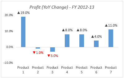
Color Negative Chart Data Labels in Red with downward arrow

Make your Excel charts easier to read with custom data labels Click the Chart Wizard button in the standard tool bar. Click Line under Chart Type. Click Next twice. In the Chart Title box, enter 2006 Region One Sales. Click the Legend tab, and clear the Show...

Share :